Creating a Search Engine-style Document
for NHS GP, PCN and ICB data

In my previous job experiences, I often found myself needing to reference one or more large databases for information quickly. For example, this could be for pricing of a particular product in a product list or general information about a specific customer in a customer-base. This can be a particularly time-consuming endeavour if you don't have the luxury of being able to query the data, such as in an SQL database. So, I found myself wanting to increase efficiency and productivity, whilst also being user-friendly.

So there we had our problem, how can I reference information from a database that's quick, efficient, and easy to use? I immediately thought, "wouldn't it be great if I could just Google the information I wanted?". Well, as it turns out, I could replicate the action of Googling something in Excel.

Before we get ahead of ourselves, I first needed to collect all of the data I required and collate it into one big database. For the purposes of this project, I used the open source databases on GPs, PCNs and ICBs provided by NHS Digital. The link for all the datasets used can be found at the top of this page by clicking the "Datasets" button. The specific datasets I used in this project are listed below:

• General Practice Data - epraccur
• PCN Data - epcn
• ICB Data - eccg

Now that I have all of the datasets, I compiled the information I wanted into one large dataset. To do this, I utilised the VLOOKUP function. This data is particularly well suited for the VLOOKUP function because each PCN and each ICB has a code which is unique to each individual entity. So, all I would need to do is match the relevant code from the GP data, to the codes in the PCN and ICB data and return the information I wanted. In this instance, the information I wanted to return was the name of the PCN and/or ICB. An example of the VLOOKUP function in action from the document can be seen below:

=VLOOKUP([@[Commissioner Code]],Codes,2,FALSE)

In the formula above, I'm looking for the value in each cell of the the column called "Commissioner Code", and trying to match that value to a value in the lefthand column of the table called "Codes". If a match is found, the formula will display the value of the cell in the 2nd column in the corresponding row where the match was found i.e., the name of the PCN or ICB. If no match is found, "#N/A" will be displayed instead. The "FALSE" part of the function specifies the type of lookup/match. Here, FALSE indicates that we only want EXACT MATCHES i.e. both the lookup cell value and the matched cell value are identical.

By utilising the VLOOKUP function, I now have a master dataset with all of the information I require. From here, I can start to build my "search engine".

In order to build my search engine, I need two parts to work together. The first is a search bar, where the user can input what they want to search for. The second is a formula that will search the database we've compiled based on the contents of the search bar, and return all relevant results. Lets first create a search bar. In order to create the search bar in Excel, you're going to want to make sure you have the relevant settings enabled. The setting you're going to need is the "Developer" tab in the ribbon. You can enable this from your Excel workbook by going to File>Options>Customise Ribbon, from here, on the righthand side, you should see the Developer option with a checkbox next to it. If not already, make sure this option is ticked and then confirm this by pressing "Ok". You should now have the Developer tab on your ribbon.

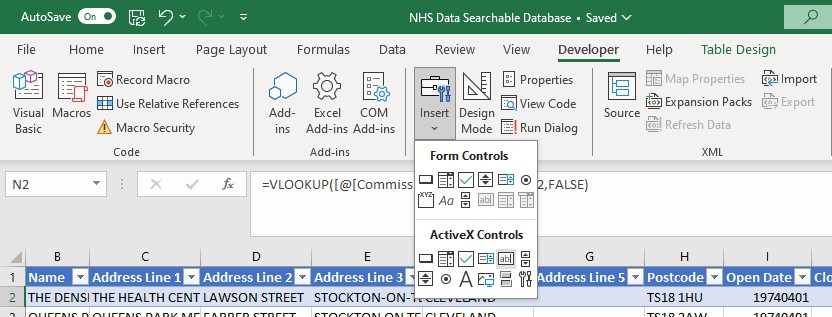
To create a search bar, go to the Developer tab on the ribbon and click the "Insert" button. You should see a dropdown menu as shown in the picture above. Under "ActiveX Controls" select the "text box" option. From here you simply have to click and drag to create your text box. However, the text box in this format doesn't do anything. In order to make the text box interactable with the Excel worksheet we have to link the text box to a cell in the workbook. To do this, we have to be in "Design Mode" which is next to the "Insert" button under the Developer tab of the ribbon. In Design Mode, we're going to right-click the text box and select "Properties", which will open the following window:

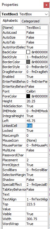
From the Properties menu, look for "Linked Cell". In the Linked Cell box, type the cell reference of the cell you wish to link to the text box e.g. B16. Now that we have done this step, the text box is linked to the cell we've specified, in this instance cell B16. What this means is that anything we type in the text box, will be mirrored in cell B16. This is great because now we have a way of referencing the contents of the search bar in a formula. From here, it's time to write a formula that is going to search the database we created and return any relevant results to the contents of the search bar. The formula I used in the document is shown below:

=FILTER(GP,ISNUMBER(SEARCH(B16,GP[Organisation Code]))+ISNUMBER(SEARCH(B16,GP[Name]))+ISNUMBER(SEARCH(B16,GP[Address Line 1]))+ISNUMBER(SEARCH(B16,GP[Address Line 2]))+ISNUMBER(SEARCH(B16,GP[Address Line 3]))+ISNUMBER(SEARCH(B16,GP[Address Line 4]))+ISNUMBER(SEARCH(B16,GP[Address Line 5]))+ISNUMBER(SEARCH(B16,GP[Postcode]))+ISNUMBER(SEARCH(B16,GP[Commissioner Name]))+ISNUMBER(SEARCH(B16,GP[Contact Telephone Number]))+ISNUMBER(SEARCH(B16,GP[Prescribing Setting]))+ISNUMBER(SEARCH(B16,GP[PCN Name])))

Well that looks like a monstrosity...

When dealing with long formulas, I always find it helps to break them down into its component parts. Lets start by identifying the functions used in the formula:

• FILTER
• ISNUMBER
• SEARCH

Lets start with the FILTER function. The purpose of this function in this formula is to remove any irrelevant information from the search result and only return information that is linked to what is contained in the search bar. The structure of the FILTER function is (array,include,if_empty). Looking at the formula above, the array specified is the table called "GP", this is what I have called our database in the document. The "include" section of the FILTER function is actually the remainder of the formula and the "if empty" component is omitted as it is optional. Therefore, lets move on to the next function, ISNUMBER.

The ISNUMBER function is exactly what it sounds like, it checks if a specified value is a number and returns TRUE or FALSE depending on the outcome. This doesn't sound like it would be useful here, however when combined with the SEARCH function, it actually enables us to return multiple results. So lets look at the remaining function, SEARCH.

Excel defines the SEARCH function as "Returns the number of the character at which a specific character or text string is first found, reading left to right (not case-sensitive)". In our formula, the SEARCH function is searching for the value of B16 i.e. the search bar, in the columns specified in the database. If a match is found, this function will return a number. Again, at face-value this doesn't sound helpful to what we want to achieve. So now that we know what each component is doing, lets put this all together to try and understand how this formula works.

To understand fully, lets go in reverse order starting with the SEARCH function. As mentioned above, if a match is found between the contents of the search bar and the specified column in the database, the SEARCH function will return a number. The important thing to note here is that, if there is no match, a number is not returned. Next, the ISNUMBER function returns TRUE or FALSE based on whether the specified value is a number. Because the value we have specified the ISNUMBER function to evaluate is the SEARCH function, this now means the all matches are labelled as "TRUE" and non-matches are labelled "FALSE". Lastly, the FILTER function tallies all of the "TRUE" values, filters out any rows of data that return a "FALSE" value and returns the values in the rows that a corresponding to a "TRUE" value.

Whew!... That was a lot to take in but I think the formula used in this project is a great example of the versality Excel can provide!

Lastly, I'd like to conclude by going all the way back to the original question that promoted this project in the first place, "how can I reference information from a database that's quick, efficient, and easy to use?". Hopefully now at the end of this project, everyone can answer this question to some extent. I encourage everyone to download the document and have a play around yourself. I personally found that this document answered the original problem I had. Typing something into a search bar is something we're all intimately familiar with and ticks that user-friendly requirement. Also, when typing in the search bar, the results appear in real-time infront of you thus, satisfying the criteria for speed and efficiency.

I hope you all enjoyed reading this project as much as I enjoyed making it! Please feel free to have a go yourself. If anyone has any questions regarding this project, you can reach out to me on LinkedIn using the links provided at the top of this page.

Thank you all for reading!